Sustainability Economics

“Operation Ranch Hand” (1962-1971) used aerial-spary (of defoliants and herbicides) to prevent Viet Cong from using food and vegetation cover for their ambush. The procurement of chemicals for the spray, particularly, napalm from the Dow Chemical and Agent Orange from Monsanto, Hercules Inc. (and a few more companies) was objected by 17 nobel laureates, 5000 other scientists and numerous thinktanks of those times. However, what is less known is that numerous shareholders in the market also came together to oppose the production of these chemicals; a one-of-the-first modern example of the practice of “responsible investment”, where the business stakeholders began believing in the importance of ethical investments, and of caring deeply about the environmental, social, and governance (ESG) considerations of investment decisions in a business. This incidence is also a precursor to the concept of ESG investment (Roncalli 2024, p. 3). During this operation, in November 1967, a famous “political action”, well-known amongst the mathematics community, came into limelight – a daring initiative by Prof. Alexander Grothendieck (then at IHES) to deliver lectures on topics, like, functional analysis, homological algebra, sheaf theory, algebraic topology, and Weil conjectures. The lectures were delivered to about fifty people in the University of Hanoi, Vietnam, near the forests. Understandably, there was a looming threat of the American chemical weapons that could have invaded the Vietnamese grounds, and to deliver “mathematical lectures” under such sensitive conditions, is now (historiographically) documented as a humanitarian response of a mathematician to opppose the loss of lives caused by the US-Vietnam war. I attempt to also classify this as an investment that underscores how “Mathematics” transcends international disputes and conflicts, and does not seem too distant from other humanitarian investments such as ESG.

Post-war witnessed a growth in socially responsible investment decisions, such as the famous example of Moskowitz 1972 publishing a list of socially responsible stocks, like Chase Manhattan, Johnson products, Levi Strauss, New York Times, Whirlpool, and Xerox (Roncalli 2024, p. 3), albeit they underperformed the Dow Jones. Extending the socially responsible investment to sovereigns and countries, a more recent example of US “Sudan Accountability and Divestment Act” (Dec. 2007) witnessed the leeway to state/local government to divest assets in companies engaging in Sudanese business operations that include oil-related, military, mineral-extraction activities during the War in Darfur (Roncalli 2024, p. 4).

Another famous example of ESG-style investment framework, which could be seen as a multi-national extension of the country or corporate level ESG, is the United Nations Framework on Climate Change (UNFCCC). UNFCCC is one of the many conventions which falls under the supreme governing body of an international convention called Conference of Parties (COP) (active since 1995) and famously known for the international treaties – Kyoto Protocol (1997) and the Paris Agreement (2015) – on abating the harmful global effects of climate change.

In an ongoing struggle to limit the global warming to 1.5 °C, which, by the ongoing release of 41.6 Gt carbon emissions every year will deplete the current carbon budget of 200 Gt by 2030, there have been numerous scientific proposals to NOT overshoot the limit. The key proposal is that of facilitating finance flows of up to $2 trillion a year from developed to developing countries. In fact, Boltan and Kleinnijenhuis (2024) suggested an economic framework to calculate the “social cost of carbon” to quantify the economic returns from this (climate) financing: another calculation goes by promising a return of 182%, if developed nations provide $2.8 trillion for emissions mitigation in developing countries, the expected ecnonomic benefits are at least $ 7.9 trillions (still limited to developed nations).

Before uncovering the implications of this paper, let us uncover some of the key mathematical and qualitative concepts often used in the literature of “climate finance”, hugely borrowed from a freshly-released book by Thierry Roncalli, Université Paris-Saclay (Handbook of Sustainable Finance 2024). Interested readers are kindly redirected to the fresh release of this book for further details.

Mathematics of Climate Finance

ESG Scoring – model, algorithm, and structure

Let us denote an ESG score by $S$ , which take values between $S^{-}$ and $S^{+}$ , such that higher the $S$ , the “good” the risk is and the lower the $S$ , the “bad” is the risk. These adjectives can help one in finding a threshold above which a “selection” of the group and below which an “exclusion” of the group is preferable. However, the same model helps in calculation of the scores and in the choice of threshold, leading one to an endogeneous problem. To get rid of this issue, different frameworks of calculations are adoped: (i) clustering and classification using unsupervised statistical method to construct ESG scores, (ii) adapting the result to a binary (good versus bad) statistical model. Once the selection of “good risks” is performed, the scores are calculated using the procedure discussed below.

A multi-level non-overlapping graph, also called a “tree”, is used to compute ESG scores. This is because the inherent properties of a tree: (a) no cycles (closed loop within the graph), (b) $n$ nodes have $n-1$ edges, (c) minimally connected (removing an edge will break the graph in two pieces)

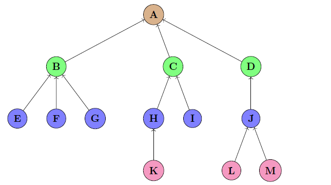
are just right enough to model the “bottom-up” calculation of ESG scores. An example calculation is as follows: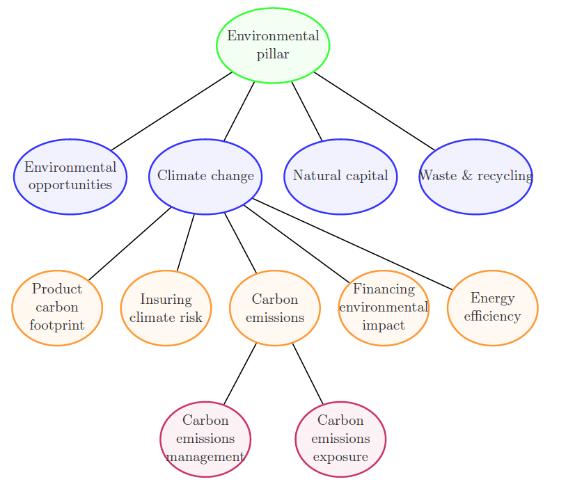

The lowest (level 4) level is made of two metrics: carbon emissions management and carbon emission exposure which combine to form carbon emissions (level 3). Four more metrics in level 3, other than carbon emissions, combine to form the climate change metric in level 2. Three more metrics come together to form the level 1 metric environmental pillar.
Impact Investing

There is a big difference between value and values. Decision-making of some investors and managers is driven by financial value, whilst that of others is driven by non-pecuniary preferences or values. This leads to two broadly opposite methods of investing: investing with impact and investing for impact, such that in the former, one looks for values after value, and in the latter, one looks for values before value. In fact, the entire spectrum of impact ecosystem can be summarised in the following schematic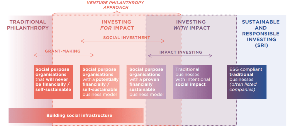

where one can see that traditional philanthrophy and Sustainable-Responsible Investing lie on the opposite ends. It is also crucial to note that the degree of intentionality and the active risk taken by investors vary in with and for investments.
Climate Change in the history of mathematics

The mathematical history of climate change can be traced back to the French mathematician Joseph Fourier who published Remarques générales sur les températures du globe terrestre et des espaces planétaires in 1824 (translated here), where he calculated that the Earth should be not as warm, theoretically, as it is now, based on its size and distance from the Earth. Three effects were accounted for in his calculation of Earth’s temperature, namely, sun’s rays, irradiation by stars, and some heat the Earth retains within itself. Fourier cited work (1774) by Genevan scientist Horace Bénédict de Saussure (1774) who found that a dark box with glass pane when exposed to the sun gets heated up by several degrees in comparison to the outside temperature (coined as the greenhouse effect). Fourier realised based on Bénédict work that the Earth’s atmosphere is responsible for this effect which keeps the Earth warmer because “heat in the state of light meets with less resistance in penetrating the air than in returning to the air when it is converted into non-luminous heat” (Roncalli 2024, p. 453).

In another paragraph, Fourier notes that, “The presence of the atmosphere produces an effect of the same sort, but which, in the present state of theory and owing further to lack of observations with which theory may be compared, cannot yet be exactly defined. However great the effect may be, one would not suppose that the temperature caused by the incidence of the rays of the Sun on an extremely large solid body would greatly exceed that which one would observe on exposing a thermometer to the light of that star” (RTP 2004 translation, p.5). The original French text is here:

On a side-note, the readers are welcome to point me to library/archive centre where original edition of this article is kept.
Explicit expression for the carbon budget

We compute the carbon budget $\mathcal{CB}$ under different carbon emission reduction assumptions. The carbon emissions at time $t$ are denoted as $\mathcal{CE}(t)$ .

Case 1: Assuming that the reduction rate is constant and linear, such that

$\mathcal{R}(t_0, t) = \mathcal{R}(t - t_0)$ , the carbon budget is given by
$\mathcal{CB}(t_0, t) = \int_{t_0}^t \left( \mathcal{CE}(t_0) - \mathcal{R}(s - t_0) \right) ds$ .

Upon integration, the final solution is given by
$\mathcal{CB}(t_0, t) = (t - t_0) \mathcal{CE}(t_0) - \frac{(t - t_0)^2}{2} \mathcal{R}$

Case 2: Assuming that there is constant compound reduction rate, one obtains

$\mathcal{CE}(t) = (1 - \mathcal{R})^{(t - t_0)} \mathcal{CE}(t_0)$

The carbon budget can be calculated as
$\mathcal{CB}(t_0, t) = \mathcal{CE}(t_0) \int_{t_0}^t (1 - \mathcal{R})^{(s - t_0)} ds$

which upon integration yields
$\mathcal{CB}(t_0, t) = \mathcal{CE}(t_0) \frac{(1 - \mathcal{R})^{(t - t_0)} - 1}{\ln(1 - \mathcal{R})}$ .

Case 3: Exponential Decay of Emissions
Assuming that the emissions decay exponentially at rate $\mathcal{R}$ ,
$\mathcal{CE}(t) = e^{-\mathcal{R}(t - t_0)} \mathcal{CE}(t_0)$ ,

the carbon budget is:
$\mathcal{CB}(t_0, t) = \mathcal{CE}(t_0) \int_{t_0}^t e^{-\mathcal{R}(s - t_0)} ds$

which upon integration yields
$\mathcal{CB}(t_0, t) = \mathcal{CE}(t_0) \frac{1 - e^{-\mathcal{R}(t - t_0)}}{\mathcal{R}}$
Portfolio decarbonisation

To construct a portfolio $w$ with a low carbon metric (carbon intensity), fund managers often use a reference portfolio $b$ which measures the reduction $\mathcal{R}(w|b)$ , where $b$ could be a model portfolio, capital weighted benchmark, or an old managed portfolio. As a result, the portfolio management constraint can be written as

$\mathcal{CI}(w) \leq (1-\mathcal{R}) \mathcal{CI}(b)$

where $\mathcal{CI}$ is the carbon intensity. Though reduction in carbon intensity, or portfolio decarbonisation, could be seen as an application of portfolio optimisation, it is a difficult exercise in practice, and can be seen as an exclusion process within the category of exclusion ESG strategies. A hidden form of divestment, the action of portfolio decarbonisation impacts the worst-in-class issuers with high carbon intensities (Roncalli 2024, p. 803).

The detailed optimisation problem is defined as

$w^{\star} = [\arg \min \frac{1}{2} (w - b)^\top \Sigma (w - b)]\quad \text{s.t.} \quad\begin{cases} \mathbf{1}_n^\top w = 1, \ w \in \Omega, \ \mathbf{0}_n \leq w \leq \mathbf{1}_n, \ \mathcal{CI}(w) \leq (1 - \mathcal{R}) \mathcal{CI}(b) \end{cases}$

where portfolio $w$ closely “tracks” the benchmark $b$ in terms of returns by minimising the covariance matrix of the asset returns given by $\Sigma$ , and overall, the minimising the track error variance given by $w^{*}$ given above. The constraints defined above mean that the sum of weights is 1 (all capital is fully invested), no shortselling is allowed for the stocks, and the weights $w$ satisfy additional constraints $\Omega$ .

In fact, as discussed in Roncalli 2024, p. 803, it is possible to eliminate $m$ worst performing stocks by introducing a statistic $\mathcal{CI}_{m,n}$ which is the (n−m+1)-th lowest carbon intensity value in the sorted list of carbon intensities. The portfolio weights $w_{i}$ for the $m$ worst carbon intensity assets are set to zero, such that stocks with carbon intensity values below $\mathcal{CI}_{m,n}$ remain in the portfolio. The updated portfolio optimisation problem is given as

$w^{\star} = [\arg \min \frac{1}{2} (w - b)^\top \Sigma (w - b)] \quad \text{s.t.} \quad \begin{cases} \mathbf{1}_n^\top w = 1, \ w \in \Omega, \ \mathbf{0}_n \leq w \leq \mathbf{1}_n \, { \mathcal{CI} < \mathcal{CI}^{(m,n)} }\end{cases}$