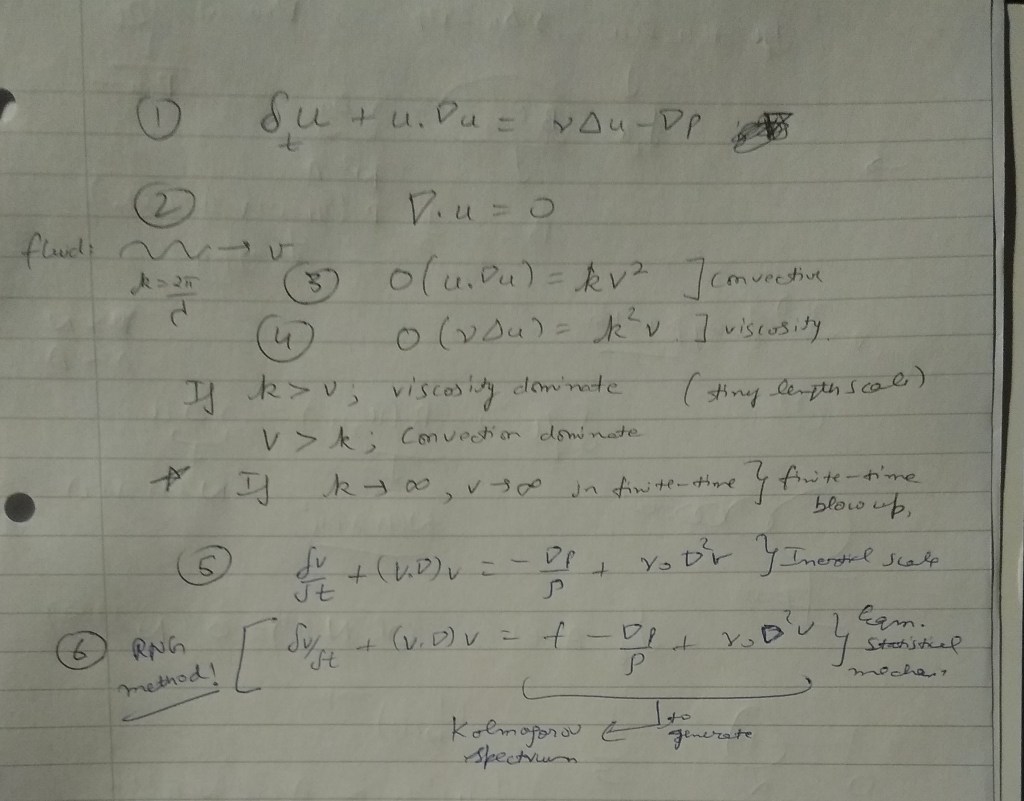
In NS equations, non-linear term dominate viscosity term when order of velocities is higher than wavenumber (3). For lower velocity, viscosity term dominate (4). Non-linear terms are coupled (across different length scales), hence onset of turbulence causes distribution of velocities across all frequency domains. It can be understood on performing Fourier transform of NS and transferring from spatial to wavenumber space. Coupling of different wavelengths cause Re to increase for smaller wavelengths and cause instabilities. As a result, velocity lowers at smaller scales; viscous regime dominates. But if viscous regime completely take over, velocity will reduce to zero ultimately, which is absurd. Hence, velocity has to concentrate largely in a small space – which is called intermittency; outside that space, it is zero. Now, intermittency is a belief. It is assumed because one needs a way to account for the scenario where bounds of velocities/vorticities upon space and time averages are broken – since, it is a possibility that hasn’t been ruled out rigorously. There could be another creation – something other than intermittency possible though, to account for the violation of velocity bounds. Original K41 didn’t account for intermittency. Self-similar blowup of solutions (solution concentrated in a spatial ball of radius ~ (T-Tc)^{0.5}) has been ruled out as well [1]. Let’s first talk about a typical “intermittency” approach undertaken by man functional analysts.
Another length scale, of burst when velocity bound is violated and intermittency accounts for that, has to be found out. So, two length scales – Kolmogorov and below that (leading to burst) are important.
In this article, I will be discussing how bounds on gradient of velocities in various dimensions have been used to find any length scale, smaller than Kolmogorov, if possible [2].
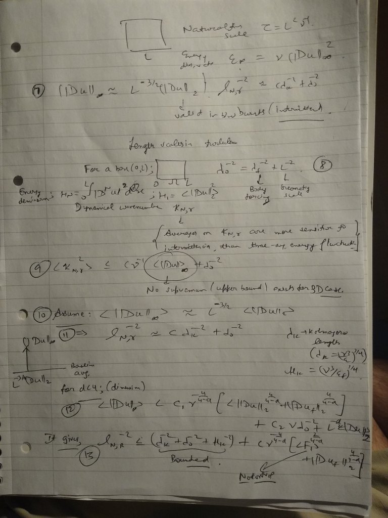
The geometry chosen is a box of length L, which sets a natural time scale,
Now, the whole quest is to find different length scales and relate them with differential of velocities. Eqn. (8) shows how length scales from geometry and body forcing couple together to form \lambda_0. Eqn. (9) shows how dynamical wavenumber is bounded by the length scale \lambda_0 and <||Du||>_\infty (which is theoretical, infinitely differentiable velocity field). There is no upper bound existing for this term in 3D case. Hence, one has to start assumption as given in Eqn. (10) where <||Du||>_\infty is approximated to <||Du||>_2 (two-times differentiable). This assumption gives another length scale (Eqn. (11)) which is combination of Kolmogorov and \lambda_0 length scale. Now, a relaxation of this assumption by moving to higher-order differential d of velocity field can be performed. It is done in Eqn. (12) and (13). Ultimately, length scale is shown to be a combination of bounded terms (Kolmogorov, \lambda_0 and Kolmogorov with forcing –\mu_k) and terms with coefficent of -4. One doesn’t have much control on the latter term (<F_1>, and it can grow out of control.
Hence, ultimately, there are three major classes of length scales. First, is Kolmogorov scale which can be derived from assumption (10), assumed velocity second-order differentiable. When the intermittent event/burst occurs, length scales smaller than Kolmogorov are possible, however there is no means to express those length scales – as <F_1> grow out of bound. This is because when <F_1> grows out of bound and singular at finite time. In the equilibrium case, when bursts haven’t occured, the time-average of velocities can reach supremum and length scales smaller than Kolmogorov. However, which scales become active isn’t possible to investigate with the analysis above. Above analysis is an indication of what can happen as opposed to what will happen.
There are various singularities of Euler equations in 3D case which have been shown to be impossible:
i) Kinks or curvature singularities in vortex lines.
ii) Vorticity shocks when vorticity becomes discontinuous though bounded.
iii) Rate of strain matrix becomes singular while vorticity remains bounded.
DNS of turbulence might cause such formations, but these would be a numerical artifact.
Enstrophy, which is the ratio of energy dissipation rate and viscosity, is an important parameter. It is being argued that it may remain bounded and still the Euler equations develop singualrity. Hence, monitoring ||\omega_\infty|| is important and will be discussed in another blog post. Also, quest for smaller scales than Kolmogorov is unfulfilled, hence more literature search will be performed. On top of all, the belief of intermittency should be always kept in mind, which means other procedures to express intermittencies (geometrically, computationally) should never be overlooked – atleast, Tao’s program of discretely self-similar programs is following that approach (will discuss in another blog post). In addition, Nash embeddings have been recently shown to derive turbulence in fluid flows, by De Lellis and others [3]. This area will also be understood in broad-detail.
References:
2. Doering, C., & Gibbon, J. (1995). Regularity and length scales for the 2d and 3d Navier-Stokes equations. In Applied Analysis of the Navier-Stokes Equations (Cambridge Texts in Applied Mathematics, pp. 137-156). Cambridge: Cambridge University Press. doi:10.1017/CBO9780511608803.008
